Hypothesis testing
Notes
Investigating a population
Deductions about the characteristics of a population can be made using a representative sample drawn from the population.
This procedure starts with a statement regarding the population and information from the sample is used to decide whether or not there is enough evidence to conclude that this statement might be false.
The null hypothesis
The initial statement about the population (the null hypothesis) is very specific.
For the case of a single sample it needs to describe the population, introduce the characteristic under study, include a statistical measure of interest (e.g. the mean) and propose an assumed value for this measure.
For instance, in a community study of systolic blood pressure an appropriate null hypothesis might be:

In raising doubts about the null hypothesis, it would be unreasonable to demand a sample mean of exactly 120 mm Hg in order to conclude that a population mean of 120 mm Hg might be plausible. The issue is whether the difference between the sample and population means is sufficiently large to cast doubt on the null hypothesis.
For example, a sample mean of 119 mm Hg might be compatible with the null hypothesis above whereas a sample mean of 105 mm Hg would raise considerable doubts.
The test statistic
Once the null hypothesis has been formulated, the next step is to analyse the data from the sample and see how far the sample observations appear to depart from what might be expected should the null hypothesis be true.
The assessment is carried out using what is known as a ‘test statistic’.
This is calculated via a formula appropriate for the null hypothesis being tested. Generally, the test statistic is equal to zero if the information from the sample completely matches what would be expected were the null hypothesis to be correct. A small value for the test statistic shows that the information from the sample is somewhat different to what might have been expected under the null hypothesis; a large value for the test statistic indicates that the sample is providing results that would be unlikely were the null hypothesis to be true.
If the sample consists of just one group and the characteristic of interest is the mean of a continuous variable such as systolic blood pressure, an appropriate test statistic is obtained using the one-sample t-test.

This is based on the sample mean divided by the standard error of the sample mean; for a sample mean the standard error is the standard deviation divided by the square root of the sample size. The ratio calculated is often referred to as t, which is why the test is referred to as a t-test.
The P-value
Once the test statistic has been calculated from the sample, it is necessary to work out the probability of obtaining a test statistic value of this size or greater were the null hypothesis to be true.
This probability is called the P-value for the hypothesis test.
For the one-sample t-test, the P-value is the probability of obtaining a sample mean at least as divergent as the one in the study (relative to its standard error) from the assumed population mean. If the observed scenario is unlikely then there is evidence against the null hypothesis. Rarely, the P-value is equal to 1. In this situation the sample mean is equal to the population mean.
The smaller the P-value, the stronger is the evidence against the null hypothesis. This evidence should be described as strong, moderate, weak, etc., leaving the reader or audience to decide whether or not the null hypothesis is plausible. This goes against the long tradition in medical research of concluding that a null hypothesis should be rejected because the P-value is less than 0.05 and otherwise accepted. In exploratory studies, P-values just above 0.05 can be useful in identifying leads for further research.
The 95% confidence interval
The standard error of the sample mean can be used to calculate a range of plausible values for the population mean.
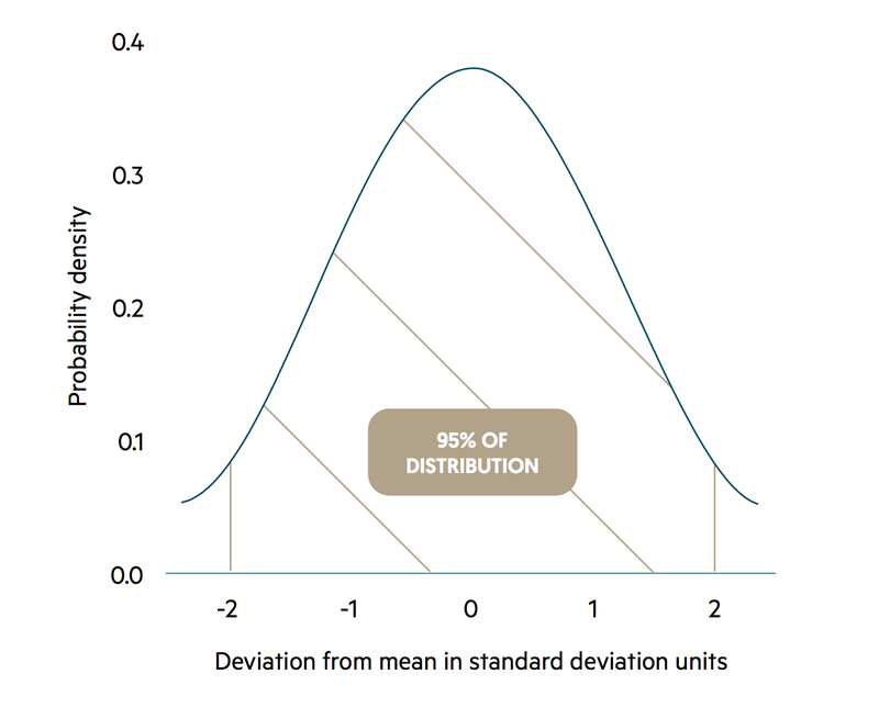
It can be shown that there is a 95% chance of the population mean being in the range of sample mean minus 1.96 standard errors (lower limit) to sample mean plus 1.96 standard errors (upper limit). This is known as a 95% confidence interval.
The value of 1.96 in the calculation of the confidence interval arises because to a good degree of approximation the standard error follows a Normal distribution and 95% of such a distribution lies within 1.96 standard deviations from the mean.
Assumption
Various assumptions need to be made when hypothesis testing is carried out.
For the one-sample t-test, the sample should be representative of the population; if this is not so it is difficult to take account of the sample bias even using sophisticated statistical methods of analysis.
The measurements in the sample are taken to be independent of each other. If the values of some observations are influenced by those of the remainder more advanced statistical techniques for correlated data are required. In addition, observations should be Normally distributed in the population. For instance, populations with a highly skewed distribution should not be subjected to this test. If any of these assumptions are not met there is a risk of obtaining misleading P-values.
Statistical significance
If the strength of evidence against a null hypothesis gives a P-value of less than 0.05, the null hypothesis value is implausible and not contained within the 95% confidence interval. This type of finding is often described as being of statistical significance.
Clinical importance
An issue that is often overlooked in hypothesis testing is that of clinical importance.
The 95% confidence interval for a finding that has statistical significance may contain points that are so close to the null hypothesis value that the difference is unimportant from a clinical aspect. The minimum difference to be taken as clinically important should be stated prior to the hypothesis testing taking place. For a blood pressure study this minimum difference might be 5 or 10 mm Hg. In order for a finding to trigger changes in management, all points within the 95% confidence interval should indicate a difference from the null hypothesis value that is of clinical importance.
Examples
Suppose that for the community study of systolic blood pressure with the null hypothesis “In the population of adults living in this community, the mean systolic blood pressure is equal to 120 mm Hg” a minimum difference of 5 mm Hg is considered to be of clinical importance. In other words, mean SBP values indicating a clinically important difference are either no more than 115 or no less than 125 mm Hg.
- 95% confidence interval from 113 to 119 mm Hg
Statistically significant finding. The null hypothesis value (120) is not within the confidence interval. Some values (e.g. 114) represent a difference of clinical importance.
- 95% confidence interval from 117 to 124 mm Hg
This finding is not of statistical significance. The null hypothesis value (120) is contained within the confidence interval. No difference is of clinical importance.
- 95% confidence interval from 107 to 114 mm Hg
Statistically significant and clinically important finding. The null hypothesis value (120) is not contained within the confidence interval. In addition, all differences are of clinical importance as values in the confidence interval are less than 115 mm Hg.
Other applications of hypothesis testing
These notes are just a brief, introductory look at hypothesis testing and only considers the case of a continuous variable for one sample.
Hypothesis testing can be extended to many more contexts including the analysis of two or more groups, binary and ordered variables, and associations between continuous variables.
Last updated: September 2017
Have comments about these notes? Leave us feedback